Generalized Linear Models
GEO 200CN - Quantitative Geography
Professor Noli Brazil
April 22, 2026
In the past couple of labs we’ve learned how to run and interpret linear regression models. Linear regression models are used when your outcome is a continuous numeric variable. Generalized Linear Models (GLM’s) are extensions of linear regression to areas where assumptions of normality and homoskedasticity do not hold. There are several versions of GLM’s, each for different types and distributions of outcomes. In this lab, we will focus on outcomes that are binary (Yes or No) or are counts of events. We use logistic regression to model the former, and poisson regression to model the latter. The objectives of this lab are as follows
- Learn how to run and evaluate a logistic regression model
- Learn how to run and evaluate a poisson regression model
To help us understand the logistic regression model, we will examine the association between landslide occurrence and various environmental factors in the San Pedro Creek Watershed in Pacifica, CA. To help us understand the poisson regression model, we will examine the association between the number of hurricane occurrences in the United States between 1851 and 2010 and various environmental variables. We’ll be closely following the material presented in Handout 5.
Installing and loading packages
We introduce one new package in today’s lab
install.package("lmtest")Load this package along with others we need.
library(tidyverse)
library(lmtest)
Logistic regression
In many situations in your work as a Geographer, your outcome will be coded as a binary variable (1 or 0; Yes or No). You can use a linear regression to model a binary outcome, but you’ll typically break the assumption of homoskedastic residuals and you may get predictions outside of 1 or 0. That’s why you’ll need to turn to logistic regression to model the relationship.
Bring in the data
Download the file landslides.csv from Canvas in the Week 4 Lab and Assignment folder. Bring in the file in
landslides <- read_csv("landslides.csv")The data contain various locations in the San Pedro Creek Watershed in Pacifica, CA. The main goal of the analysis is to examine the characteristics that are associated with landslide occurrence. Landslides were detected on aerial photography from 1941, 1955, 1975, 1983, and 1997, and confirmed in the field during a study in the early 2000’s. We’ll create a logistic regression to compare landslide probability to various environmental factors. We’ll use elevation elev, slope slope, hillshade hillshade, distance to nearest stream stD, distance to nearest trail trD, and the results of a physical model predicting slope stability as a stability index SI.
Our research question is: What environmental characteristics are associated with landslide occurrence?
We will be diving into spatial data next lab, but that should not
stop us from doing some rudimentary mapping. Specifically, we have
latitude and longitude points for each location in the dataset, so we
can map the data using our good friend ggplot(). We’ll
indicate which area experienced a landslide or not using the variable
IsSlide. We need to convert it to a factor to “color” it as a
categorical.
ggplot(landslides) +
  geom_point(mapping = aes(x = lon,
                           y = lat, col = as.factor(IsSlide))) +
  xlab("Longitude") +
  ylab("Latitude") +
  labs(color = "Landslide")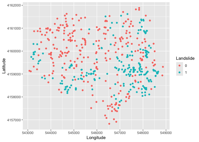
Simple Logistic Regression
We first examine the distribution of our binary dependent variable IsSlide. We create a bar chart showing the distribution of the landslide indicator.
landslides %>%
  group_by(IsSlide) %>%
  summarize (n = n()) %>%
  mutate(freq = n / sum(n))  %>%
  ggplot() +
    geom_bar(mapping=aes(x=as.factor(IsSlide), y=freq),stat="identity") +
    xlab("Landslide")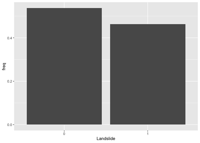
Let’s now run a logistic regression model. We’ll start simple,
regressing IsSlide on slope. Instead of using the
function lm() to run a logistic regression model as we did
when running linear regression models, we will use the function
glm(), which stands for Generalized Linear Models.
glm() is similar to lm(), but gives us the
option of a variety of families to use in fitting the model (the shape
that we hypothesize represents the shape of the function f that
defines the relationship between Y and X).
We specify a family by using the argument family =. If
we wanted a standard linear regression, which assumes a normal
distribution, family will equal gaussian
(fancy word for normal). For a list of glm families, check
the help documentation ? glm. We use
family = binomial for a logistic regression.
logit1.fit <- glm(IsSlide ~ slope,
                  family = binomial,
                  data = landslides)
We can summarize the modelling results using summary().
The resulting output is very similar to the output from
lm().
summary(logit1.fit)##
## Call:
## glm(formula = IsSlide ~ slope, family = binomial, data = landslides)
##
## Coefficients:
## Estimate Std. Error z value Pr(>|z|)
## (Intercept) -3.39142 0.37008 -9.164 <2e-16 ***
## slope 0.13471 0.01387 9.715 <2e-16 ***
## ---
## Signif. codes: 0 '***' 0.001 '**' 0.01 '*' 0.05 '.' 0.1 ' ' 1
##
## (Dispersion parameter for binomial family taken to be 1)
##
## Null deviance: 668.29 on 483 degrees of freedom
## Residual deviance: 513.54 on 482 degrees of freedom
## AIC: 517.54
##
## Number of Fisher Scoring iterations: 5Question 1: What is the interpretation of the slope coefficient?
Let’s compare our results to those from an OLS regression model. An
OLS for a binary response variable is known as a linear probability
model. We use glm() again, but this time use the (default)
Gaussian distribution.
ols.land <-glm(IsSlide ~ slope,
              family = gaussian,
              data = landslides)
and a summary
summary(ols.land)##
## Call:
## glm(formula = IsSlide ~ slope, family = gaussian, data = landslides)
##
## Coefficients:
## Estimate Std. Error t value Pr(>|t|)
## (Intercept) -0.076552 0.044594 -1.717 0.0867 .
## slope 0.023734 0.001767 13.429 <2e-16 ***
## ---
## Signif. codes: 0 '***' 0.001 '**' 0.01 '*' 0.05 '.' 0.1 ' ' 1
##
## (Dispersion parameter for gaussian family taken to be 0.181679)
##
## Null deviance: 120.331 on 483 degrees of freedom
## Residual deviance: 87.569 on 482 degrees of freedom
## AIC: 552.06
##
## Number of Fisher Scoring iterations: 2Question 2: What is the interpretation of the slope coefficient in ols.land?
You can create a plot like the one showed in Handout 5 (right hand
plot) by predicting the probability of a landslide for given values of
slope. The minimum and maximum slope for our data set are 0 and
42.29, respectively, so let’s predict landslide occurrence for slopes
between 0 to 43 using the predict() function. The function
below tells R to give predicted landslide occurrence for values of
slope between 0 and 43.
pfit1 <- predict(logit1.fit,
                 slope = c(0:43))
In predicting using a regression model, you can either predict landslides for the 484 observations in the original data set or predict for a new set of observations. In the code above, we are predicting for a new set of observations - areas with slopes between 0 and 43 - i.e. 0, 1, 2, 3 … 41, 42, and 43.
Let’s get a summary of our predicted values
summary(pfit1)## Min. 1st Qu. Median Mean 3rd Qu. Max.
## -3.3914 -1.1843 0.0494 -0.3301 0.7812 2.3059We get values ranging from -3.4 to 2.3. But, these are not
probabilities. Remember, as described in the handout, the response
variable is modeled as a logit, so R will give us logits in return. To
convert the logit to a probability, use the argument
type = "response" inside predict()
pfit1 <- predict(logit1.fit,
                 data.frame(slope = c(0:43)),
                 type = "response")
summary(pfit1)
## Min. 1st Qu. Median Mean 3rd Qu. Max.
## 0.03256 0.12543 0.37882 0.42496 0.72158 0.91692The predicted probability of a landslide ranges from 3.3% to 91.7%.
Question 3: Create a plot similar to the one shown in this week’s handout (right hand plot) showing the predicted probabilities from logit1.fit and the observed data.
Question 4: Create a plot similar to the one shown in this week’s handout (left hand plot) showing the predicted probabilities from ols.land and the observed data.
Multiple Logistic Regression
We now move to the multiple logistic regression framework by adding more than one independent variable. Let’s add the variable hillshade, which is a categorical variable (High, Mid, and Low).
logit2.fit <- glm(IsSlide ~ slope + hillshade,
                  family = binomial,
                  data = landslides)
summary(logit2.fit)
##
## Call:
## glm(formula = IsSlide ~ slope + hillshade, family = binomial,
## data = landslides)
##
## Coefficients:
## Estimate Std. Error z value Pr(>|z|)
## (Intercept) -3.18010 0.44451 -7.154 8.42e-13 ***
## slope 0.14545 0.01582 9.195 < 2e-16 ***
## hillshadeLow -0.92891 0.30165 -3.079 0.00207 **
## hillshadeMid -0.49244 0.27044 -1.821 0.06862 .
## ---
## Signif. codes: 0 '***' 0.001 '**' 0.01 '*' 0.05 '.' 0.1 ' ' 1
##
## (Dispersion parameter for binomial family taken to be 1)
##
## Null deviance: 668.29 on 483 degrees of freedom
## Residual deviance: 503.68 on 480 degrees of freedom
## AIC: 511.68
##
## Number of Fisher Scoring iterations: 5Let’s calculate the predicted probability of a landslide at each value of hillshade, holding the slope at its mean. We need to create a data frame containing the values for slope and hillshade that we want to predict for. What are the categories of hillshade?
table(landslides$hillshade)##
## High Low Mid
## 121 121 242Let’s save these categories in a vector.
hillshade <- c("High", "Mid", "Low")Now you need to create a data frame containing the vector
hillshade we created above as one column and the overall mean
of slope as another column (name the column slope
because it needs to match the variable name used in the prediction
model). So you should have a 3 x 2 data frame. Then plug this data frame
into the predict() function following what we did
earlier.
Question 5: What is the difference in the probability of a landslide between a Low hillshade area and a High hillshade area holding the slope at its mean?
Handout 5 goes through the various ways we can interpret logistic regression coefficients. We already went through a few above. What about the odds ratio interpretation?
Question 6: Convert the logit2.fit coefficients to interpret them as the change in the odds ratio with a one unit increase in the independent variables. For a one unit increase in slope, the odds of a landslide (versus no landslide) increase by a factor of what amount?
Goodness of fit
The Handout goes through measures of best fit for a logistic regression model. Fortunately, some of these measures are reported in the model summary. Let’s run a multiple logistic regression model adding more variables to the model. Below, we’ve added curvature, elevation, distance to the nearest stream, and distance to the nearest trail.
logit3.fit<- glm(IsSlide ~ slope + hillshade + curv + elev + stD + trD,
                 family = binomial,
                 data = landslides)
How does this model compare to one that also includes the slope stability index?
logit4.fit<- glm(IsSlide ~ slope + hillshade + curv + elev + stD + trD + SI,
                 family = binomial,
                 data = landslides)
Executing summary() on these results will give us some
but not all of the fit measures discussed in the handout. The likelihood
ratio test can be run using the function lrtest(), which is
part of the lmtest package. The function allows you
compare the fit between two different models.
Question 7: Based on the fit measures discussed in the handout, which model, logit3.fit and logit4.fit, provides the best fit? Explain why.
Poisson regression
Rather than the continuous numeric outcome for the linear regression model or the binary outcome for the logistic regression model, the poisson regression model is used for discrete count variables as outcomes. Common examples of these types of responses include species count data in ecology, the number of crimes in sociology, and the number of respondents or patients reporting a side-effect or symptom of interest in health studies.
Bring in the data
Download the file hurricanes.csv from Canvas in the Week 4 Lab and Assignment folder. Bring in the file in.
hurricanes <- read_csv("hurricanes.csv")The data contain the number of hurricanes occurring in the US (excluding Hawaii) by year (each row represents a year). The dataset also includes a number of environmental factors that have been shown to contribute to hurricane formation and intensity. Higher sea surface temperatures (SST) has been associated with hurricane formation. This is because the warm ocean water provides sensible heat and water vapor that fuels the intense convection of a hurricane, and assists the conversion of a cold-core tropical depression to a warm-core cyclone.
The Southern Oscillation Index (SOI) is defined as the normalized sea-level pressure difference between Tahiti and Darwin,indicating El Niño (negative SOI) or La Niña (positive SOI) phases, which heavily influence global hurricane activity. Negative SOI (El Niño) reduces Atlantic hurricane activity due to high wind shear but increases Eastern Pacific activity. Conversely, positive SOI (La Niña) enhances Atlantic hurricanes.
The North Atlantic Oscillation (NAO) is a atmospheric pressure pattern that influences hurricane tracks and intensity. A negative NAO phase often leads to more hurricanes in the Gulf of Mexico, while a positive NAO typically directs storms towards the U.S. East Coast
The Sunspot Number (SSN) is a measure of solar activity that influences hurricane formation by affecting temperatures and sea surface conditions. Generally, fewer hurricanes occur in the Atlantic when sunspots are numerous (high SSN), as increased UV radiation during solar maximums stabilizes the atmosphere, inhibiting storm development.
Our research question is: What environmental characteristics are associated with the number of hurricanes in a given year?
Multiple Poisson Regression
Let’s first check the distribution of our outcome variable.
hurricanes %>%
  ggplot() +
    geom_histogram(aes(x=All), binwidth=1) +
    xlab("Number of Hurricanes")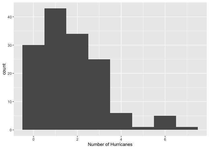
The distribution is lower bounded at zero, shows discrete values, and shows the typically Poisson-like left-leaning skewed shape.
Let’s run an OLS regression model.
ols.hur <-glm(All ~ SOI + NAO + SST + SSN,
              family = gaussian,
              data = hurricanes)
And the results
summary(ols.hur)##
## Call:
## glm(formula = All ~ SOI + NAO + SST + SSN, family = gaussian,
## data = hurricanes)
##
## Coefficients:
## Estimate Std. Error t value Pr(>|t|)
## (Intercept) 1.886895 0.187610 10.058 < 2e-16 ***
## SOI 0.113878 0.040247 2.829 0.00535 **
## NAO -0.292870 0.117255 -2.498 0.01366 *
## SST 0.431398 0.492961 0.875 0.38301
## SSN -0.003939 0.002378 -1.656 0.09995 .
## ---
## Signif. codes: 0 '***' 0.001 '**' 0.01 '*' 0.05 '.' 0.1 ' ' 1
##
## (Dispersion parameter for gaussian family taken to be 1.964968)
##
## Null deviance: 316.04 on 144 degrees of freedom
## Residual deviance: 275.10 on 140 degrees of freedom
## AIC: 516.35
##
## Number of Fisher Scoring iterations: 2Let’s check the distribution of the OLS residuals to determine if it breaks some of the assumptions outlined in the OLS lab. In particular, let’s check if the errors are normally distributed.
#save the residuals
hurricanes <- hurricanes %>%
            mutate(resid = resid(ols.hur))

#check normality.
hurricanes %>%
  ggplot() +
  geom_histogram(mapping = (aes(x=resid))) +
  xlab("Absolute Residuals")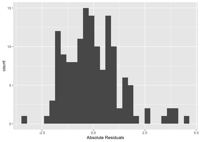
#formal test
shapiro.test(resid(ols.hur))
##
## Shapiro-Wilk normality test
##
## data: resid(ols.hur)
## W = 0.95423, p-value = 9.99e-05Looks like the residuals are not normally distributed.
Question 8: What would ols.hur predict for the number of hurricanes in a year when SOI = -3, NAO = 3, SST = 0 and SSN = 250? Why is this value problematic?
Let’s fit a poisson regression. Here, we specify
family = poisson in glm().
pois.fit <-glm(All ~ SOI + NAO + SST + SSN,
              family = poisson,
              data = hurricanes)
Examine the coefficient estimates.
summary(pois.fit)##
## Call:
## glm(formula = All ~ SOI + NAO + SST + SSN, family = poisson,
## data = hurricanes)
##
## Coefficients:
## Estimate Std. Error z value Pr(>|z|)
## (Intercept) 0.595288 0.103342 5.760 8.39e-09 ***
## SOI 0.061863 0.021319 2.902 0.00371 **
## NAO -0.166595 0.064427 -2.586 0.00972 **
## SST 0.228972 0.255289 0.897 0.36977
## SSN -0.002306 0.001372 -1.681 0.09284 .
## ---
## Signif. codes: 0 '***' 0.001 '**' 0.01 '*' 0.05 '.' 0.1 ' ' 1
##
## (Dispersion parameter for poisson family taken to be 1)
##
## Null deviance: 197.89 on 144 degrees of freedom
## Residual deviance: 174.81 on 140 degrees of freedom
## AIC: 479.64
##
## Number of Fisher Scoring iterations: 5Question 9: Transform the coefficient estimates into incident rate ratios. Interpret the statistically significant coefficients (p-values < 0.05).
To add an offset in glm(), include in the formula
offset() and the logarithm of the exposure variable.
Question 10: Should we include an offset term in pois.fit? If yes, what variable might we include (that’s not in the data set)? If no, then why not?

This
work is licensed under a
Creative
Commons Attribution-NonCommercial 4.0 International License.
Website created and maintained by Noli Brazil