Introduction to R
GEO 200CN - Quantitative Geography
Professor Noli Brazil
March 30, 2026
We will be using R to complete all data analysis tasks in this class. For those who have never used R or it has been a long time since you’ve used the program, welcome to what will be a life fulfilling journey! The goal of this class is not to learn skills to be a programmer. Instead, we are going to learn enough of R to apply the statistical methods we will learn in the class using real data.
The objectives of the guide are as follows:
- Download R and RStudio
- Get familiar with the RStudio interface
- Understand R data types
- Understand R data structures, in particular vectors and data frames
- Understand R functions
- Understand R packages
- Understand R Markdown and the process for submitting assignments
What is R?
R is an environment for data analysis and graphics. R is an interpreted language, not a compiled one. This means that you type something into R and it does what you tell it. It is both a command line software and a programming environment. It is an extensible, open-source language and computing environment for Windows, Macintosh, UNIX, and Linux platforms, which allows for the user to freely distribute, study, change, and improve the software. It is basically a free, super big, and complex calculator. You will be using R to accomplish all data analysis tasks in this class. You might be wondering “Why in the world do we need to know how to use a statistical software program?” Here are the main reasons:
We will be going through a lot of equations and abstract concepts in lecture and readings. Applying these concepts using real data is an important form of learning. A statistical software program is the most efficient (and in many cases the only) means of running data analyses, not just in the cloistered setting of a university classroom, but especially in the real world. Applied data analysis will be the way we bridge statistical theory to the “real world.” And R is the vehicle for accomplishing this.
In order to do applied data analysis outside of the classroom, you need to know how to use a statistical program. There is no way around it as we don’t live in an exclusively pen and paper world. If you want to collect data on soil health, you need a program to store and analyze that data. If you want to collect data on the characteristics of recent migrants, you need a program to store and analyze that data. Even in qualitative work, after you’ve transcribed your interviews, the information you collected are data, which you will then need a software program to store and analyze that data.
The next question you may have is “I love Excel [or insert your favorite program]. Why can’t I use that and forget your stupid R?” Here are some reasons
- it is free. Most programs are not;
- it is open source. Which means the software is community supported. This allows you to get help not from some big corporation (e.g. Microsoft with Excel), but people all around the world who are using R. And R has a lot of users, which means that if you have a problem, and you pose it to the user community, someone will help you;
- it is powerful and extensible (meaning that procedures for analyzing data that don’t currently exist can be readily developed);
- it has the capability for mapping data, an asset not generally available in other statistical software;
- If it isn’t already there, R is becoming the de-facto data analysis tool in the physical and social sciences
R is different from Excel in that it is generally not a point-and-click program. You will be primarily writing code to clean and analyze data. What does writing or sourcing code mean? A basic example will help clarify. Let’s say you are given a dataset with 10 rows representing people living in Davis, CA. You have a variable in the dataset representing individual income. Let’s say this variable is named inc. To get the mean income of the 10 people in your dataset, you would write code that would look something like this
mean(inc)The command tells the program to get the mean of the variable
inc. If you wanted the sum, you write the command
sum(inc).
Now, where do you write this command? You write it in a script. A script is basically a text file. Think of writing code as something similar to writing an essay in a word document. Instead of sentences to produce an essay, in a programming script you are writing code to run a data analysis. The basic process of sourcing code to run a data analysis task is as follows.
- Write code. First, you open your script file, and
write code or various commands (like
mean(inc)) that will execute data analysis tasks in this file. - Send code to the software program. You then send your some or all of your commands to the statistical software program (R in our case).
- Program produces results based on code. The program then reads in your commands from the file and executes them, spitting out results in its console screen.
I am skipping over many details, most of which are dependent on the type of statistical software program you are using, but the above steps outline the general work flow. You might now be thinking that you’re perfectly happy pointing and clicking your mouse in Excel (or wherever) to do your data analysis tasks. So, why should you adopt the statistical programming approach to conducting a data analysis?
- Your script documents the decisions you made during the data analysis process. This is beneficial for many reasons.
- It allows you to recreate your steps if you need to rerun your analysis many weeks, months or even years in the future.
- It allows you to share your steps with other people. If someone asks you what were the decisions made in the data analysis process, just hand them the script.
- Related to the above points, a script promotes transparency (here is what i did) and reproducibility (you can do it too). When you write code, you are forced to explicitly state the steps you took to do your research. When you do research by clicking through drop-down menus, your steps are lost, or at least documenting them requires considerable extra effort.
- If you make a mistake in a data analysis step, you can go back, change a few lines of code, and poof, you’ve fixed your problem.
- It is more efficient. In particular, cleaning data can encompass a lot of tedious work that can be streamlined using statistical programming.
Getting R
Although you can use campus labs to run R, it is best to download it on your computer so you can access it at any time. R can be downloaded from one of the “CRAN” (Comprehensive R Archive Network) sites. In the US, the main site is at http://cran.us.r-project.org/. Look in the “Download and Install R” area. Click on the appropriate link based on your operating system.
If you already have R on your computer, make sure you have the most updated version of R on your personal computer (R 4.5.2 “[Not] Part in a Rumble”).
Mac OS X
On the “R for macOS” page, there are multiple packages that could be downloaded. If you have a Mac with Apple Silicon, click on R-4.5.2-arm64.pkg; if you don’t have Silicon and are running on macOS 11 (Big Sur) or higher, click on R-4.5.2-x86_64.pkg; if you are running an earlier version of OS X, download the appropriate version listed under “Binaries for legacy macOS/OS X systems.”
After the package finishes downloading, locate the installer on your hard drive, double-click on the installer package, and after a few screens, select a destination for the installation of the R framework (the program) and the R.app GUI. Note that you will have to supply your computer’s Administrator’s password. Close the window when the installation is done.
An application will appear in the Applications folder: R.app.
Browse to the XQuartz download page. Click on the most recent version of XQuartz to download the application.
Run the XQuartz installer. XQuartz is needed to create windows to display many types of R graphics: this used to be included in MacOS until version 10.8 but now must be downloaded separately.
Windows
On the “R for Windows” page, click on the “base” link, which should take you to the “R-4.5.2 for Windows” page
On this page, click “Download R 4.5.2 for Windows”, and save the exe file to your hard disk when prompted. Saving to the desktop is fine.
To begin the installation, double-click on the downloaded file. Don’t be alarmed if you get unknown publisher type warnings. Window’s User Account Control will also worry about an unidentified program wanting access to your computer. Click on “Run” or “Yes”.
Select the proposed options in each part of the install dialog. When the “Select Components” screen appears, just accept the standard choices (the default). For Startup options, keep the default.
Note: Depending on the age of your computer and version of Windows, you may be running either a “32-bit” or “64-bit” version of the Windows operating system. If you have the 64-bit version (most likely), R will install the appropriate version (R x64 3.5.2) and will also (for backwards compatibility) install the 32-bit version (R i386 3.5.2). You can run either, but you will probably just want to run the 64-bit version.
What is RStudio?
If you click on the R program you just downloaded, you will find a very basic user interface. For example, below is what I get on a Mac
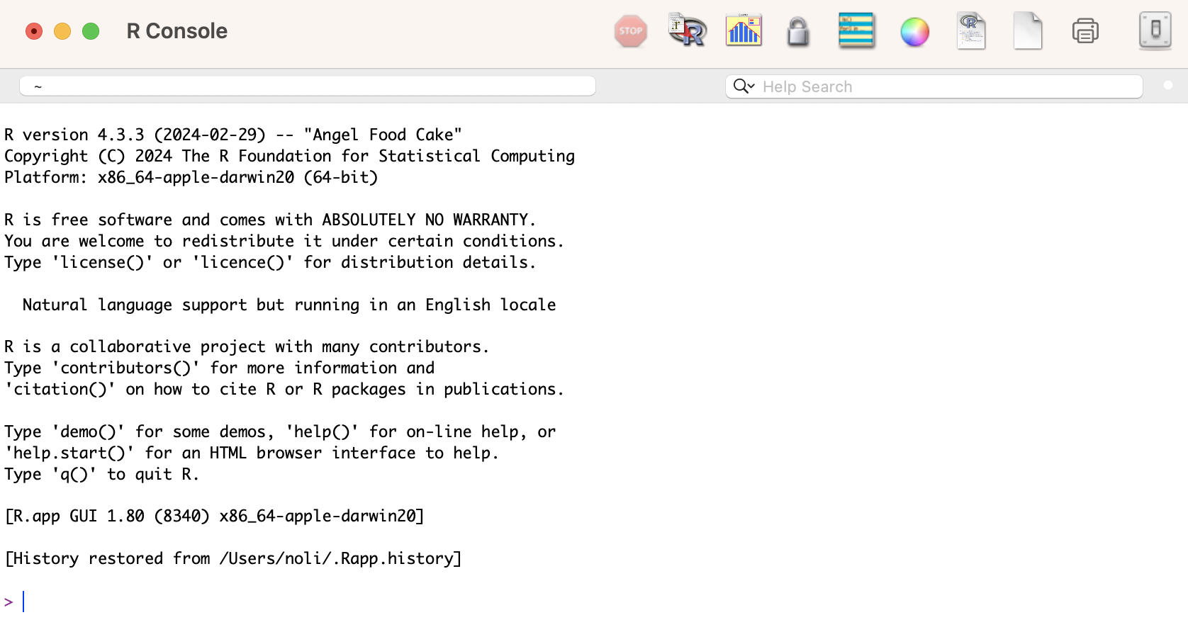
We will not use R’s direct interface to run analyses. Instead, we will use the program RStudio. RStudio gives you a true integrated development environment (IDE), where you can write code in a window, see results in other windows, see locations of files, see objects you’ve created, and so on. To clarify which is which: R is the name of the programming language itself and RStudio is a convenient interface.
Getting RStudio
To download and install RStudio, follow the directions below
- Navigate to RStudio’s download site
- Click on the “Download RStudio Desktop” link under the header “2: Install RStudio”. This will prompt you to save an installer package on your drive.
- Click on the installer that you downloaded. Follow the installation wizard’s directions, making sure to keep all defaults intact. After installation, RStudio should pop up in your Applications or Programs folder/menu.
Note that the most recent version of RStudio works only for certain operating systems (OS). If you have an older OS, you will need to download an older version RStudio, which you can find here.
The RStudio Interface
Open up RStudio. You should see the interface shown in the figure below, which has three windows.
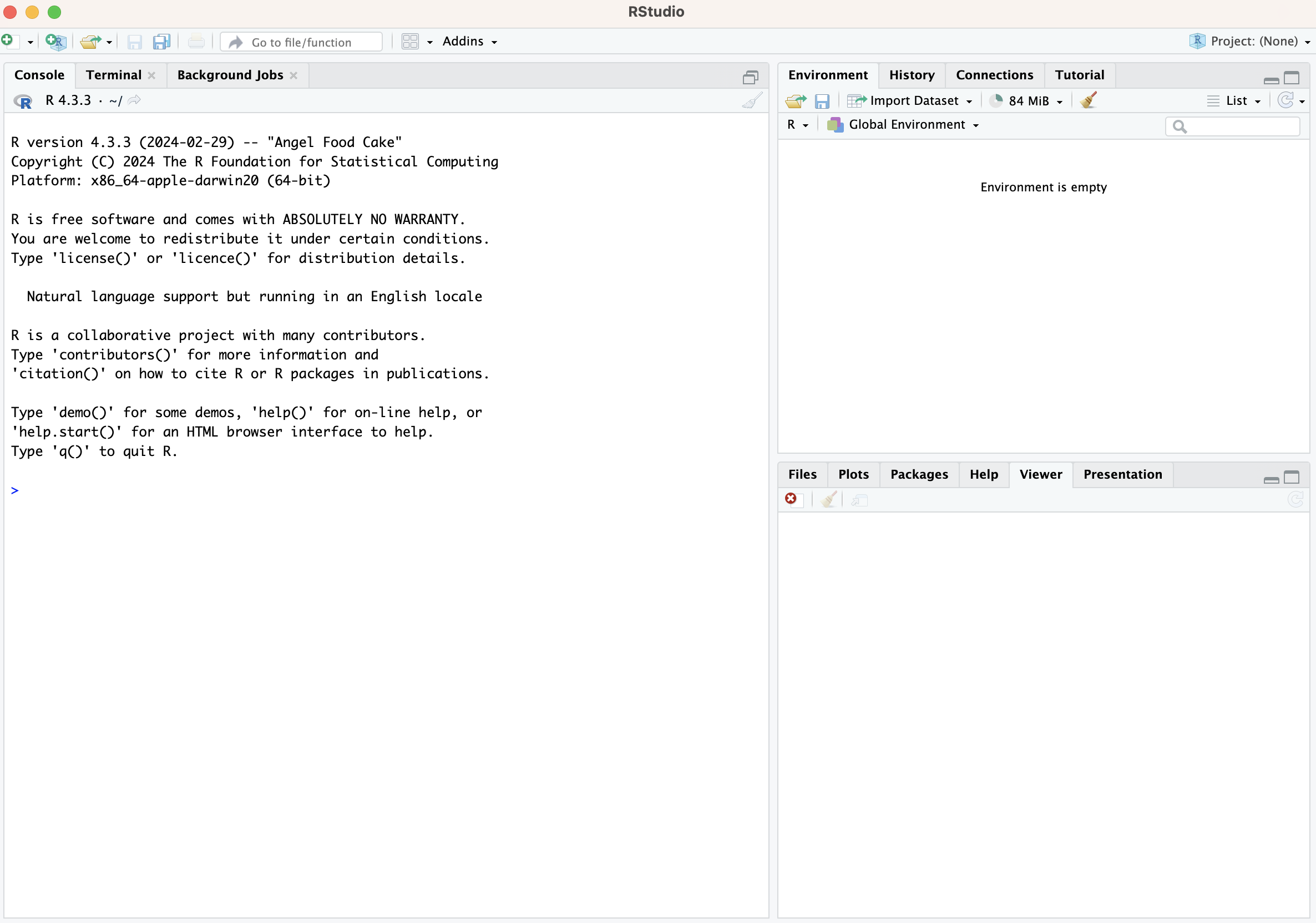
- Console (left) - The way R works is you write a
line of code to execute some kind of task on a data object. The R
Console allows you to run code interactively. The screen prompt
>is an invitation from R to enter its world. This is where you type code in, press enter to execute the code, and see the results. - Environment, History, and Connections tabs
(upper-right)
- Environment - shows all the R objects that are
currently open in your workspace. This is the place, for example, where
you will see any data you’ve loaded into R. When you exit RStudio, R
will clear all objects in this window. You can also click on
 to clear out all the objects loaded and created in your current
session.
to clear out all the objects loaded and created in your current
session. - History - shows a list of executed commands in the current session.
- Connections - you can connect to a variety of data
sources, and explore the objects and data inside the connection. I
typically don’t use this window, but you can.
- Tutorial - used to run tutorials that will help you
learn and master the R programming language.
- Environment - shows all the R objects that are
currently open in your workspace. This is the place, for example, where
you will see any data you’ve loaded into R. When you exit RStudio, R
will clear all objects in this window. You can also click on
- Files, Plots, Packages, Help and Viewer tabs
(lower-right)
- Files - shows all the files and folders in your current working directory (more on what this means later).
- Plots - shows any charts, graphs, maps and plots
you’ve successfully executed (we’ll be using this window starting in Lab
5).
- Packages - tells you all the R packages that you have access to (more on this in Lab 2).
- Help - shows help documentation for R commands that
you’ve called up.
- Viewer - allows you to view local web content (won’t be using this much).
- Presentation - used to display HTML slides.
There is actually fourth window. But, we’ll get to this window a little later (if you read the assignment guidelines you already know what this fourth window is).
For more information on each tab, check this resource.
Using R
Let’s now explore what R can do. R is really just a big fancy
calculator. For example, type in the following mathematical expression
next to the > in the R console (left window)
1+1Note that spacing does not matter: 1+1 will generate the
same answer as 1 + 1. Can you say hello to the
world?
hello world## Error in parse(text = input): <text>:1:7: unexpected symbol
## 1: hello world
## ^Nope. First, if you are beginner to programming, get used to errors like the one we just saw. Frustration is a natural reaction when you start programming in R because it is such a stickler for punctuation, and even one character out of place can cause it to complain. But while you should expect to be a little frustrated, take comfort in that this experience is typical and temporary: it happens to everyone, and the only way to get over it is to keep trying
Whenever you get an error, ask yourself: What is the problem here? In this case, we need to put quotes around it.
"hello world"## [1] "hello world"“hello world” is a character and R recognizes characters only if there are quotes around it. Characters are one of R’s five basic data types. The most important basic (or “primitive”) data types are the “numeric” (for numbers) and “character” (for text) types. Additional types are the “integer”, which can be used to represent whole numbers; the “logical” for TRUE/FALSE, and the “factor” for categorical variables. These are all discussed below.
Data Types
Character values
A character variable is used to represent letters, codes, or words.
Character values are often referred to as a “string”. We designate
values as characters by placing either single or double quotes around
it. There is no difference in behavior. I recommend always using double
quotes, unless you want to create a string that contains multiple double
quotes. We already went through one example of a character when we wrote
in the words “Hello world” above. If you forget to close a quote, you’ll
see +, the continuation character. The + tells you that R
is waiting for more input; it doesn’t think you’re done yet. Usually,
this means you’ve forgotten either a ” or a ). Either add the missing
pair, or press ESCAPE to abort the expression and try again.
You might think that the value “1” is a number. Well, with quotes around, it isn’t! Anything with quotes will be interpreted as a character. No ifs, ands or buts about it.
R has a set of base functions that manipulate strings. For example,
to get a part of a string use the function substr()
substr("Hello World", 1, 5)## [1] "Hello"The code above keeps the character values in the 1st through 5th positions of the word “Hello World”. Try using other numbered positions and see what you get.
To replace characters in a string use the function
gsub().
gsub("Hello", "Bye bye", "Hello World")## [1] "Bye bye World"Here, the function finds the set of characters in the first value “Hello”, replaces it with the second value “Bye bye”, in all instances in the third value “Hello World”.
Numeric values
Numerics are separated into two types: integer and double. The
distinction between integers and doubles is usually not important. R
treats numerics as doubles by default because it is a less restrictive
data type. You can do any mathematical operation on numeric values. We
added one and one above. We can also multiply using the *
operator.
2*3## [1] 6Divide
4/2## [1] 2And even take the logarithm!
log(1)## [1] 0log(0)## [1] -InfUh oh. What is -Inf? Well, you can’t take the logarithm
of 0, so R is telling you that you’re getting a non numeric value in
return. The value -Inf is a special numeric value
representing a result too large to be stored, typically produced by
dividing a non-zero number by zero, or taking the log of 0.
Logical values
A logical takes on two values: FALSE or TRUE. Think of a logical as the answer to a question like “Is this value greater than (lower than/equal to) this other value?” The answer will be either TRUE or FALSE. For example, typing in the following
3 > 2## [1] TRUEyields a TRUE value. You are asking R, is 3 greater than 2?
We can test for equality using two equal signs == (not a
single = which would be assigning a value).
"clare" == "jonathan"## [1] FALSE<= means “smaller or equal” and >=
means “larger or equal”.
2 <= 2## [1] TRUE3 <= 2## [1] FALSEFactor values
A factor is a nominal (categorical) variable with a set of known
possible values called levels. They can be created using the
as.factor() function. In R you typically need to convert
(cast) a character variable to a factor to identify groups for use in
statistical tests and models. We’ll go through factor values in more
depth later in the course.
Missing values
All basic data types can have “missing values”. A missing value
represents data that is unknown, unmeasured, or unavailable. These are
represented by the symbol NA for “Not Available”. Typing NA
in the R Console yields
NA## [1] NANote that NA is not quoted (it is a special symbol, it
is not the word “NA”).
Properly treating missing values is very important. The first
question to ask when they appear is whether they should be missing (or
did you make a mistake in the data manipulation?). If they should be
missing, the second question becomes how to treat them. Can they be
ignored? Should the records with NAs be removed?
Data Structures
You just learned that R has several basic data types. Now, let’s go through how we can store data in R. That is, you type in the character “hello world” or the number 3, and you want to store these values so you can use them later. You do this by using R’s various data structures.
Vectors
A vector is the most common and basic R data structure and is pretty
much the workhorse of the language. A vector is simply a sequence of
values which can be of any data type but all of the same type. There are
a number of ways to create a vector depending on the data type, but the
most common is to insert the data you want to save in a vector into the
command c(). For example, to represent the values 4, 16 and
9 in a vector type in
c(4, 16, 9)## [1] 4 16 9You can also have a vector of character values
c("diana", "clare", "gwen")## [1] "diana" "clare" "gwen"The above code does not actually “save” the values 4, 16, and 9 - it
just prints it on the screen in a vector. If you want to use these
values again without having to type out c(4, 16, 9), you
can save it in a data object. You assign data to an object using the
arrow sign <-. This will create an object in R’s memory
that can be called back into the command window at any time. For
example, you can save “hello world” to a vector called b by
typing in
b <- "hello world"You can pronounce the above as “b becomes ‘hello world’”. Note that the value of b is not printed, it’s just stored. If you want to view the value, type b in the console.
b## [1] "hello world"Note that R is case sensitive, if you type in B instead of b, you will get an error. Lets save the numbers 4, 16 and 9 into a vector called v1
v1 <- c(4, 16, 9)
v1
## [1] 4 16 9How do you know you’ve created these objects for later use? You should see the objects b and v1 pop up in the Environment tab on the top right window of your RStudio interface.
Note that the name v1 is nothing special here. You could have named the object x or geo200cn or your pet’s name (mine was didi). You can’t, however, name objects using special characters (e.g. !, @, $) or only numbers (although you can combine numbers and letters, but a number cannot be at the beginning e.g. 2d2). For example, you’ll get an error if you save the vector c(4,16,9) to an object with the following names
123 <- c(4, 16, 9)
!!! <- c(4, 16, 9)
## Error in parse(text = input): <text>:2:5: unexpected assignment
## 1: 123 <- c(4, 16, 9)
## 2: !!! <-
## ^You want your object names to be descriptive, so you’ll need to adopt
a convention for multiple words. I recommend snake_case, where you
separate lowercase words with _.
Also note that to distinguish a character value from a variable name, it needs to be quoted. “v1” is a character value whereas v1 is a variable. One of the most common mistakes for beginners is to forget the quotes.
brazil## Error:
## ! object 'brazil' not foundThe error occurs because R tries to print the value of object
brazil, but there is no such object in your current
environment. So remember that any time you get the error message
object 'something' not found, the most likely reason is
that you forgot to quote a character value. If not, it probably means
that you have misspelled, or not yet created, the object that you are
referring to. I’ve included common pitfalls and R tips in this class resource.
Basic arithmetic on numeric vectors is applied to every element of the vector:
v1*2## [1] 8 32 18You can add vectors with the same length
c <- 1:5
d <- 6:10
c+d
## [1] 7 9 11 13 15You can also test their equality
c == d## [1] FALSE FALSE FALSE FALSE FALSEEvery vector has two key properties: type and
length. The type property indicates the data type that the
vector is holding. Use the base command typeof() to
determine the type
typeof(b)## [1] "character"typeof(v1)## [1] "double"Note that a vector cannot hold values of different types. If
different data types exist, R will coerce the values into the highest
type based on its internal hierarchy: logical < integer < double
< character. Type in test <- c("r", 6, TRUE) in your
R console. What is the vector type of test?
The command length() determines the number of data
values that the vector is storing
length(b)## [1] 1length(v1)## [1] 3You can also directly determine if a vector is of a specific data
type by using the command is.X() where you replace
X with the data type. For example, to find out if
v1 is numeric, type in
is.numeric(b)## [1] FALSEis.numeric(v1)## [1] TRUEThere is also is.logical(), is.character(),
is.factor(), is.infinite() and
is.na(). You can also coerce a vector of one data type to
another. For example, save the value “1” and “2” (both in quotes) into a
vector named x1
x1 <- c("1", "2")
typeof(x1)
## [1] "character"To convert x1 into a numeric, use the command
as.numeric()
x2 <- as.numeric(x1)
typeof(x2)
## [1] "double"There is also as.logical(), as.character(),
and as.factor().
An important practice you should adopt early is to keep only
necessary objects in your current R Environment. For example, we will
not be using x2 any longer in this guide. To remove this object
from R forever, use the command rm()
rm(x2)The data frame object x2 should have disappeared from the Environment tab. Bye bye!
Also note that when you close down R Studio, the objects you created above will disappear for good. Unless you save them onto your hard drive (we’ll touch on saving data in next week’s lab), all data objects you create in your current R session will go bye bye when you exit the program.
Data Frames
We learned that data values can be stored in data structures known as vectors. The next step is to learn how to store vectors into an even higher level data structure. The data frame can do this. A data frame is what you get when you read spreadsheet-like data into R. Data frames store vectors of the same length. Create a vector called v2 storing the values 5, 12, and 25
v2 <- c(5,12,25)We can create a data frame using the command
data.frame() storing the vectors v1 and
v2 as columns
data.frame(v1, v2)## v1 v2
## 1 4 5
## 2 16 12
## 3 9 25Store this data frame in an object called df1
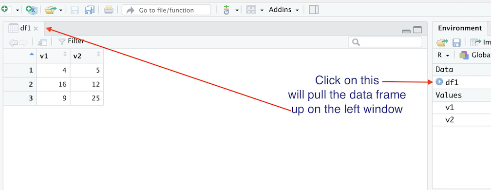
df1<-data.frame(v1, v2)df1 should pop up in your Environment window. You’ll notice
a  next to df1. This tells you that df1 possesses or
holds more than one object. Click on
and you’ll see the two vectors we saved into df1. Another neat
thing you can do is directly click on df1 from the Environment
window to bring up an Excel style worksheet on the top left of your
RStudio interface. You can’t edit this worksheet directly, but it allows
you to see the values that a higher level R data object contains.
next to df1. This tells you that df1 possesses or
holds more than one object. Click on
and you’ll see the two vectors we saved into df1. Another neat
thing you can do is directly click on df1 from the Environment
window to bring up an Excel style worksheet on the top left of your
RStudio interface. You can’t edit this worksheet directly, but it allows
you to see the values that a higher level R data object contains.
We can store different types of vectors in a data frame. For example, we can store one character vector and one numeric vector in a single data frame.
v3 <- c("diana", "clare", "gwen")
df2 <- data.frame(v1, v3)
df2
## v1 v3
## 1 4 diana
## 2 16 clare
## 3 9 gwenFor higher level data structures like a data frame, use the function
class() to figure out what kind of object you’re working
with.
class(df2)## [1] "data.frame"We can’t use length() on a data frame because it has
more than one vector. Instead, it has dimensions - the number
of rows and columns. You can find the number of rows and columns that a
data frame has by using the command dim()
dim(df1)## [1] 3 2Here, the data frame df1 has 3 rows and 2 columns. Data frames also have column names, which are characters.
colnames(df1)## [1] "v1" "v2"In this case, the data frame used the vector names for the column names.
We can extract columns from data frames by referring to their names
using the $ sign.
df1$v1## [1] 4 16 9We can also extract data from data frames using brackets
[ , ]
df1[,1]## [1] 4 16 9The value before the comma indicates the row, which you leave empty if you are not selecting by row, which we did above. The value after the comma indicates the column, which you leave empty if you are not selecting by column. Let’s select the 2nd row.
df1[2,]## v1 v2
## 2 16 12What is the value in the 2nd row and 1st column?
df1[2,1]## [1] 16We’ve been talking about the values in vectors and data frames rather abstractly. In practice, values, vectors and data frames have specific meaning in the context of data analysis. Let’s make things concrete. Take a look at this website showing crimes in California cities in 2016. Sacramento had 3,549 violent crime incidences. This is a data value (numeric!). The collection of violent crime counts for each city is a vector. The data frame has California cities as rows and the population, violent crime, homicide, and so on as columns.
Lists
A list is a very flexible container to store data. Each element of a list can contain any type of R object, e.g. a vector, matrix, data.frame, another list, or more complex data types.
Here is a simple list of three numbers
list(1:3)## [[1]]
## [1] 1 2 3It shows that the first element [[1]] contains a vector
of 1, 2, 3.
Here is one with two data types, one is a vector of two numbers and another vector of one character.
e <- list(c(2,5), 'abc')
e## [[1]]
## [1] 2 5
##
## [[2]]
## [1] "abc"Here is a list containing a vector and a data frame
list1 <- list(c, df2)
list1## [[1]]
## [1] 1 2 3 4 5
##
## [[2]]
##   v1    v3
## 1  4 diana
## 2 16 clare
## 3 9 gwenAnd a more complex list.
list2 <- list(e, df2, 'abc')
list2
## [[1]]
## [[1]][[1]]
## [1] 2 5
##
## [[1]][[2]]
## [1] "abc"
##
##
## [[2]]
## v1 v3
## 1 4 diana
## 2 16 clare
## 3 9 gwen
##
## [[3]]
## [1] "abc"We won’t run into lists too much in this class, only encountering them when we deal with spatial data. You can learn more about them and matrices, a data structure that has data frame like qualities, here.
Functions
Let’s take a step back and talk about functions (also known as
commands). An R function is a packaged recipe that converts one or more
inputs (called arguments) into a single output. We’ve already used a
number of functions above, including gsub() and all the
is.X() and as.X() commands. You execute all of
your tasks in R using functions. We have already used a couple of
functions above including typeof() and
colnames(). Every function in R will have the following
basic format
functionName(arg1 = val1, arg2 = val2, ...)
In R, you type in the function’s name and set a number of options or parameters within parentheses that are separated by commas. Some options need to be set by the user - i.e. the function will spit out an error because a required option is blank - whereas others can be set but are not required because there is a default value established.
Let’s use the function seq() which makes regular
sequences of numbers. You can find out what the options are for a
function by calling up its help documentation by typing ?
and the function name
? seqThe help documentation should have popped up in the bottom right
window of your RStudio interface. The documentation should also provide
some examples of the function at the bottom of the page. Type the
arguments from = 1, to = 10 inside the parentheses
seq(from = 1, to = 10)## [1] 1 2 3 4 5 6 7 8 9 10You should get the same result if you type in
seq(1, 10)## [1] 1 2 3 4 5 6 7 8 9 10The code above demonstrates something about how R resolves function
arguments. When you use a function, you can always specify all the
arguments in arg = value form. But if you do not, R
attempts to resolve by position. So in the code above, it is assumed
that we want a sequence from = 1 that goes
to = 10 because we typed 1 before 10. Type in 10 before 1
and see what happens. Since we didn’t specify step size, the default
value of by in the function definition is used, which ends
up being 1 in this case. How do we know what the default values are for
arguments within a function? Check the function’s help
documentation.
Each argument requires a certain type of data type. For example,
you’ll get an error when you use character values in
seq()
seq("p", "w")## Error in `seq.default()`:
## ! 'from' must be a finite numberWriting Functions
R comes with thousands of functions for you to use. Nevertheless, it is often necessary to write your own functions. For example, you may want to write a function to:
- more clearly describe and isolate a particular task in your data analysis workflow.
- re-use code. Rather than repeating the same steps several times (e.g. for each of 200 cases you are analyzing), you can write a function that gets called 200 times. This should lead to faster development of scripts and to fewer mistakes. And if there is a mistake it only needs to be fixed in one place.
For these reasons, writing functions is one of the most important
coding skills to learn. Writing your own functions is not difficult. The
below is a very simple function. It is called f. This is an
entirely arbitrary name. You can also call it
myFirstFunction. It takes no arguments, and always returns
‘hello’.
f <- function() {
    return('hello')
}
Look carefully how we assign a function to name f using
the function keyword followed by parenthesis that enclose the arguments
(there are none in this case). The body of the function is enclosed in
braces (also known as “curly brackets” or “squiggly brackets”).
Now that we have the function, we can inspect it, and use it.
f## function ()
## {
## return("hello")
## }f()## [1] "hello"f is a very boring function. It takes no arguments and
always returns the same result. Let’s make it more interesting.
f <- function(name) {
    x <- paste("hello", name)
    return(x)
}
f('Sara')
## [1] "hello Sara"Note the return statement. This indicates that variable x
(which is only known inside of the function) is returned to the caller
of the function. Simply typing x would also suffice, and ending
the function with paste("hello", name) would also do! So
the below is equivalent but shorter, at the expense of being less
explicit.
f <- function(name) {
    paste("hello", name)
}
f("Sara")
## [1] "hello Sara"Now an example of a function that manipulates numbers. This function squares the sum of two numbers.
sumsquare <- function(a, b) {
    d <- a + b
    dd <- d * d
    return(dd)
}
We can now use the sumsquare function. Note that it is
vectorized (each argument can be more than one number)
sumsquare(1,2)## [1] 9x <- 1:3
y <- 5
sumsquare(x,y)## [1] 36 49 64You can name the arguments when using a function; that often makes your intentions clearer.
sumsquare(a=1, b=2)## [1] 9But the names must match
sumsquare(a=1, d=2)## Error in `sumsquare()`:
## ! unused argument (d = 2)And both arguments need to be present
sumsquare(1:5)## Error in `sumsquare()`:
## ! argument "b" is missing, with no defaultOf course, these were toy examples, but if you understand these, you
should be able to write much longer and more useful functions. It can be
difficult to “debug” (find errors in) a function. It is often best to
first write the sequence of commands that you need outside a function,
and only when it all works, wrap that code inside of a function block
(function( ) { }).
Chapter 25 in R for Data Science provides more examples of writing your own functions.
Packages
Functions do not exist in a vacuum, but exist within R packages. Packages are the fundamental
units of reproducible R code. They include reusable R functions, the
documentation that describes how to use them, and sample data. At the
top left of a function’s help documentation, you’ll find in curly
brackets the R package that the function is housed in. For example, type
in your console ? seq. At the top right of the help
documentation, you’ll find that seq() is in the package
base. All the functions we have used so far are part of
packages that have been pre-installed and pre-loaded into R.
Many functions you will use in this class are not pre-installed. In
order to use functions in a new package, you first need to install the
package using the install.packages() command. For example,
we will be using commands from the package tidyverse
throughout the rest of this course. So, let’s install it.
install.packages("tidyverse")You should see a bunch of gobbledygook roll through your console screen. Don’t worry, that’s just R downloading all of the other packages and applications that tidyverse relies on. These are known as dependencies. Unless you get a message in red that indicates there is an error (like we saw when we typed in “hello world” without quotes), you should be fine.
Next, you will need to load packages in your working environment
(every time you start RStudio). We do this with the
library() function.
library(tidyverse)The Packages window at the lower-right of your RStudio shows you all
the packages you currently have installed. If you don’t have a package
listed in this window, you’ll need to use the
install.packages() function to install it. If the package
is checked, that means it is loaded into your current R session.
To uninstall a package, use the function
remove.packages().
Note that you only need to install packages once
(install.packages()), but you need to load them each time
you relaunch RStudio (library()). Repeat after me:
Install once, library every time. Also note that R has several packages
already preloaded into your working environment. These are known as base
packages and a list of their functions can be found here.
Tidyverse
There are two approaches to programming in R: base and tidy. Base R is the set of R tools, packages and functions that are pre-installed into R. In simple terms, it represents the building blocks of the language. Folks who learned R more than 10 or so years ago, started out in the same way you did in this lab. However, starting around 2014 or thereabouts, a new way of approaching R was born. This approach is known as tidy R or the tidyverse.
In most labs, we will be using commands from the tidyverse package. Tidyverse is a collection of high-powered, consistent, and easy-to-use packages developed by a number of thoughtful and talented R developers. The consistency of the tidyverse, together with the goal of increasing productivity, mean that the syntax of tidy functions is typically straightforward to learn. You now might be asking yourself “why didn’t he just cut straight to the tidyverse?” First, many of the topics you learned in this lab are fundamental to understanding R, tidy or not. For example, the data types remain the same whether in base or tidy world. Second, tidyverse is growing, but has not taken over. You need to know base R to do some of the data management and analysis procedures that we will be learning later in the class, particularly those that are specific to raster analysis.
With that said, my approach to this course is to lean towards the
tidy way of doing R. Tidy R is built off of base R functions, so there
is a natural connection. But, code written in the
tidyverse style is much easier to read. For example, if
you want to select certain variables from your data frame, you use an
actual tidy function named select(). For example, to
extract v1 from the data frame
df1
select(df1, v1)## v1
## 1 4
## 2 16
## 3 9In Base R, you have to use the $ sign or bracket convention shown earlier.
df1$v1## [1] 4 16 9df1[,1]## [1] 4 16 9In general, Base R has a somewhat inconsistent and sometimes incomprehensible mish-mash of function and argument styles. We’ll use both approaches, but lean more towards tidy.
R Markdown
In running the few lines of code above, we’ve asked you to work
directly in the R Console and issue commands in an interactive
way. That is, you type a command after >, you hit
enter/return, R responds, you type the next command, hit enter/return, R
responds, and so on. Instead of writing the command directly into the
console, you should write it in a script. The process is now: Type your
command in the script. Run the code from the script. R responds. You get
results. You can write two commands in a script. Run both
simultaneously. R responds. You get results. This is the basic flow.
In your homework assignments, we will be asking you to submit code in a specific type of script: the R Markdown file. R Markdown allows you to create documents that serve as a neat record of your analysis. Think of it as a word document file, but instead of sentences in an essay, you are writing code for a data analysis.
Now may be a good time to read through the class assignment guidelines as they go through the basics of R Markdown files.
After you’ve done that, answer the homework questions that are uploaded on Canvas in an RMarkdown file. Submit the R Markdown and its knitted document on Canvas by the assignment due date.

This
work is licensed under a
Creative
Commons Attribution-NonCommercial 4.0 International License.
Website created and maintained by Noli Brazil