Point Pattern Analysis

The fundamental building blocks of vector or object data are points. As such, we start our journey into spatial data analysis by going through the basic methods for examining point patterns. This guide follows closely OSU Chapter 5 and this week’s handout. The objectives of the guide are as follows

Learn spatstat package functions for setting up point data for analysis
Learn first-order or density based measures for examining point patterns
Learn second-order or distance based measures for examining point patterns
Learn the Density-Based Spatial Clustering of Applications with Noise (DBSCAN) method for locating clusters

To help us accomplish these learning objectives, we will be examining the occurrence of tornadoes in Oklahoma. This week’s assignment questions on point pattern analysis are scattered throughout this lab.

Installing and loading packages

We’ll be using a couple of new packages in this lab. First, install spatstat using install.packages(). This package contains all the functions we need to calculate the clustering methods outlined in OSU.

install.packages("spatstat")

Next, install the dbscan package. This package contains the necessary functions for running the DBSCAN method described in this week’s handout.

install.packages("dbscan")

Finally, load these and other required packages for this lab using the function library()

library(spatstat)
library(dbscan)
library(sf)
library(tidyverse)
library(RColorBrewer)

Why point pattern analysis?

Point data give us the locations of objects or events within an area. Objects can be things like trees or where an animal was last seen. They can also be houses, street lights or even people, such as the locations of where people were standing during a protest. Events can be things like the epicenter of an earthquake or where a wildfire was ignited. They can also be crimes or where someone tweeted something. Point pattern analysis can answer such questions like:

What is the density of a process? If you work on crime, you may want to find out where crime is concentrated. If you work in public health, you might want to know where the density of cholera deaths are highest.
How are points distributed across space? If you are a plant scientist, perhaps you are curious as to whether an invasive species is randomly dispersed or clustered across a study area.
Are events or objects influencing the location of other similar events or objects? Back to our crime example, you might be interested in whether a crime will trigger future crimes to occur in the same area, following a contagion effect.
Do (1)-(3) differ across some characteristic? You might be interested in whether certain crimes are more clustered than others so that you can employ different safety programs more efficiently.

You can also examine whether the density of your points covary or are influenced by other processes - such as species density and elevation.

Our research questions in this lab are: Do tornadoes cluster in Oklahoma? Where do tornadoes cluster? In the United States, tornado outbreaks have substantial effects on human lives and property. Tornado outbreaks are sequences of six or more tornadoes that are rated F1 and greater on the Fujita scale or rated EF1 and greater on the Enhanced Fujita scale and that occur in close succession. If you’re curious, here is a paper that examines tornado outbreaks in the US.

Bringing in the data

Let’s bring in a shapefile data set of tornado locations occurring in the state of Oklahoma between 2016 and 2021. Download the zip file point_pattern_lab.shp from Canvas (Week 6 - Lab and Assignment), unzip it and use st_read to read in the file.

tornado <- st_read("okl_tornado_point.shp")

The points are the initial locations of tornado touchdown. These data were derived from larger, national-level datasets generated by the National Oceanographic and Atmospheric Administration (NOAA) National Weather Service Storm Prediction Center.

Let’s also bring in a shapefile containing the boundary for the state of Oklahoma.

okla <- st_read("okl_state.shp")

To see what we got, plot the state boundary and the tornado points.

ggplot() +
  geom_sf(data = okla) +
  geom_sf(data = tornado) +
  theme_bw()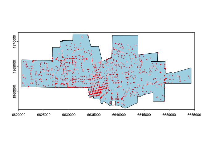

Most of the point pattern analysis tools used in this lab guide are available in the spatstat package. These tools are designed to work with points stored as ppp objects and not SpatVector or sf objects. So, yes, another spatial object to learn about. We won’t go through the nuts and bolts of how ppp objects work. We’ll cover what is only necessary for running our analyses.

We need to convert our SpatVector tornado points object into a ppp object. To do this, we use the function as.ppp(). We have to provide point coordinates and the observation window. Below we obtain the coordinates of the sf object in matrix form with st_coordinates(), and consider the observation window as the bounding box of the tornado data which can be obtained with st_bbox(). A bounding box can be used to define any area on a map. It is commonly used by mapping applications to determine which map features within a certain area should be displayed on a given map.

tornado.ppp <- as.ppp(st_coordinates(tornado), 
                      st_bbox(tornado))

As we defined above, point data give the location of objects or events within an area. In addition to coordinates, points have other data attached to them called marks. Marks are essentially attributes of the point (i.e. species of tree, type of crime). Marks could be categorical (type of crime) or continuous (diameter of tree). Right now the tornado.ppp object contains no attribute or marks information.

marks(tornado.ppp)

## NULL

Point pattern analyses should have their study boundaries explicitly defined. This is the window through which we are observing the points. One example is the boundaries of a forest if you are studying tree species distribution. In the current example, it is the boundaries of Oklahoma. spatstat uses a special boundary object - an owin, which stands for observation window. We will need to coerce okla to an object of class owin using the function as.owin().

stateOwin <- as.owin(okla)
class(stateOwin)

## [1] "owin"

To set or “bind” the state boundary owin to the tornado.ppp point feature object, use the Window() function, which is a spatstat function.

Window(tornado.ppp) <- stateOwin

We’re now set and ready to roll. Let’s do some analysis!

Centrography

Before considering more complex approaches, let’s compute the mean center and standard distance for the tornado data as described on page 125 of OSU. To calculate these values, you’ll need to extract the x and y coordinates from the tornado.ppp object using the spatstat function coords()

xy <- coords(tornado.ppp)

And then compute the mean center following equation 5.1 on page 125. We’ll use our friend summarize() to help us out here.

# mean center
mc <- xy %>%
        summarize(xmean = mean(x), 
                  ymean = mean(y))
mc

##      xmean    ymean
## 1 672303.9 57049.53

And then standard distance using equation 5.2 on page 125.

# standard distance
sd <- sqrt(sum((xy$x- mc$xmean)^2 + (xy$y - mc$ymean)^2) / nrow(xy))
sd

## [1] 190339.9

Density based measures

Centrography is rather dull because it ignores spatial variation in the data. Instead, we can explicitly examine the distribution of points across a geographic area. This is measuring first-order effects or examining point density. First-order effects or patterns look at trends over space.

Overall density

The overall density given in equation 5.3 in OSU on page 126 can be calculated as follows

StateArea <- st_area(okla)
nrow(xy) / as.numeric(StateArea)

## [1] 2.396701e-09

The command st_area(okla) calculates the area (in meters squared) of the state, which represents the value a in formula 5.3. nrow(xy) represents the number of tornadoes in the state, which represents the value n.

Overall density is a little bit better than the centrography measures, but it is still a single number, and thus we can do better. As OSU states on page 127, we lose a lot of information when we calculate a single summary statistic. Let’s go through the two “local” density approaches covered in OSU: Quadrat and Kernel density.

Quadrat counts

A basic yet descriptively useful visualization of point density is to create a grid (often called quadrats) of your study area and count the number of tornadoes in each grid cell. To compute quadrat counts (as on p.127-130 in OSU), use spatstat’s quadratcount() function. The following code chunk divides the state boundary into a grid of 3 rows and 6 columns and tallies the number of points falling in each quadrat.

qcounts1 <- quadratcount(tornado.ppp, nx= 6, ny=3)

The object qcounts1 stores the number of points inside each quadrat. You can plot the quadrats along with the counts as follows:

plot(tornado.ppp, pch=20, cols="grey70", main=NULL) 
plot(qcounts1, add=TRUE)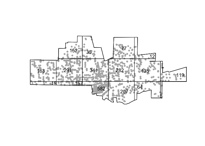

Three-by-six might be too small. Let’s instead make a 15 by 30 grid.

qcounts2 <- quadratcount(tornado.ppp, nx= 30, ny=15)

then plot

plot(tornado.ppp, pch=20, cols="grey70", main=NULL)  # Plot points
plot(qcounts2, add=TRUE)  # Add quadrat grid.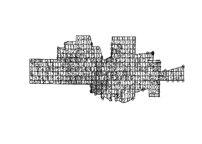

In real life one should always try a range of row and column sizes to get a sense of how sensitive the results are (this is trying to deal with the “Bad News” OSU item Scale).

We’ll need to convert the resulting qcounts2 object into a data frame to calculate the variance-mean ratio (VMR) described on page 130 in OSU.

Qcount<-data.frame(qcounts2)

And the VMR is

var(Qcount$Freq)/mean(Qcount$Freq)

## [1] 2.172899

Question 1: Explain why a VMR greater than 1 indicates spatial clustering.

Hypothesis testing

As OSU states on page 142- “It is one thing to create an index such as [the VMR]. but it is quite another to generate a significance test that answers the basic question posed at the bottom of Figure 5.14 (What can we infer about the process from the statistics?)”.

We can employ the Chi-square test for spatial randomness that OSU describes on page 142-43 using the handy dandy quadrat.test() function. The default is the Chi-square test, but you can run the Monte Carlo test described on page 148 using method = MonteCarlo.

quadrat.test(tornado.ppp, nx= 30, ny=15)

## 
##  Chi-squared test of CSR using quadrat counts
## 
## data:  tornado.ppp
## X2 = 602.05, df = 314, p-value < 2.2e-16
## alternative hypothesis: two.sided
## 
## Quadrats: 315 tiles (irregular windows)

Question 2: What are the null and alternative hypotheses for this test? What does the VMR score combined with the chi-square test tell us about the point pattern?

Kernel density

The kernel density approach is an extension of the quadrat method: Like the quadrat density, the kernel approach computes a localized density for subsets of the study area, but unlike its quadrat density counterpart, the sub-regions overlap one another providing a moving sub-region window.

The spatstat package has a function called density.ppp() that computes a kernel density estimate of the point pattern. A discussion of kernel density maps is located in page 68-71 in OSU. That discussion points to two tuning parameters that are important to consider when creating a kernel density map: the bandwidth, which controls the size and shape of the radius, and the kernel function, which controls how point counts are smoothed. We can just accept the defaults and get the following map.

ds <- density.ppp(tornado.ppp)
par(mai=c(0,0,0.5,0.5))
plot(ds, main='tornado density')

We can alter the bandwidth using the sigma = argument. A really large sigma makes the map too smooth

ds <- density.ppp(tornado.ppp, sigma = 10000)
par(mai=c(0,0,0.5,0.5))
plot(ds, main='tornado density')

A small sigma creates a map that captures really localized clusters

ds <- density.ppp(tornado.ppp, sigma = 1000)
par(mai=c(0,0,0.5,0.5))
plot(ds, main='tornado density')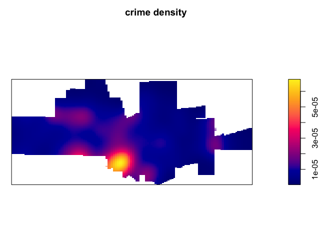

You can also change the kernel function by specifying kernel = to one of four options “gaussian” (the default), “epanechnikov”, “quartic” or “disc”.

Distance based measures

An alternative to density based methods are distance based methods whereby the interest lies in how the points are distributed relative to one another (a second-order property of the point pattern) as opposed to how the points are distributed relative to the study’s extent.

Mean Nearest-Neighbor Distance

The first distance-based method that OSU goes through is calculating the mean nearest neighbor (MNN) distance. Here, you calculate for each point the distance to its nearest neighbor. You do this using the function nndist(), which is a part of the spatstat package.

nn.p <- nndist(tornado.ppp, k=1)

We plug tornado.ppp into nndist(), resulting in a numeric vector containing the distance to each nearest neighbor (k=1 specifies distance just to the nearest neighbor. Try k= some other number and see what you get) for each point.

head(nn.p)

## [1] 12471.983  5939.146 13872.525 10581.745  6960.632  4060.785

We find that the nearest tornado to the tornado in the 1st row of tornado.ppp is 12471.983 meters We need to take the mean to get the mean nearest neighbor

mnn.p <- mean(nn.p)
mnn.p

## [1] 8704.552

The mean nearest neighbor distance of 8704.552 (check st_crs(tornado) to find how we got meters as the units of distance).

Hypothesis testing

The value 8704.552 meters seems small, indicating that tornadoes clusters. But, we can formally test this using the Clark and Evan’s R statistic described on OSU page 143. The spatstat package has the function clarkevans.test() for calculating this statistic.

clarkevans.test(tornado.ppp)

## 
##  Clark-Evans test
##  CDF correction
##  Z-test
## 
## data:  tornado.ppp
## R = 0.80667, p-value = 1.31e-14
## alternative hypothesis: two-sided

Question 3: What do the Clark Evans test results tell us about the point pattern? Explain why an R less than 1 indicates spatial clustering?

Distance Functions

The F, G, K and L functions are discussed on pages 145-148 in OSU. Our new friend spatstat provides canned functions for estimating these distributions.

The K-function summarizes the distance between points for all distances. The calculation of K consists of dividing the mean of the sum of the number of points at different distance lags for each point by the area’s density.

To compute the K function, use the function Kest().

K <- Kest(tornado.ppp)

Then plot it like on page 146 in OSU.

par(mfrow=c(1,1))
plot(K)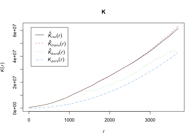

The plot returns different estimates of K depending on the edge correction chosen. By default, the isotropic, translate and border corrections are implemented. Edge corrections are discussed on pages 137-139 in OSU.

Unsurprisingly, to calculate the G, F and L functions, use the functions Gest(), Fest(), and Lest(), respectively, which take on the same form as Kest().

OSU discusses calculating envelopes around the functions to examine whether the observed functions are simply due to chance. Use the envelope() function to create the envelopes. Here, we use 99 Monte Carlo simulations.

#takes awhile
envK <- envelope(tornado.ppp, fun = Kest, nsim = 99)
plot(envK)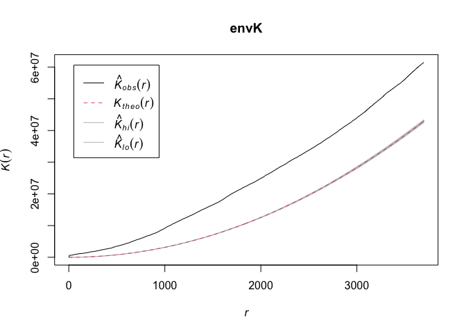

The default envelopes are the maximum and minimum values. This is set by nrank in envelope(), which is nrank=1. This means your confidence interval is

1-(2/100)

## [1] 0.98

The highest and lowest gives you two. And there are 100 K functions (99 simulations + observed K). Hence 2/100 Subtract by 1 to get the confidence level. OSU talks about the disadvantages of a simulation approach for computationally intensive calculations on page 151.

Replace Kest with Gest, Fest, and Lest to get envelopes for the other alphabet functions.

Question 4: Calculate the F and G functions. Interpret the results.

DBSCAN

The use of our techniques above are useful exploratory techniques for telling us IF we have spatial clusters present in our point data, but they are not able to tell us WHERE in our area of interest the clusters are occurring. This week’s handout covers Density-Based Spatial Clustering of Applications with Noise (DBSCAN) as a method for accomplishing this task. In DBSCAN, a cluster is defined as a collection of points that are density connected and maximize the density reachability.

To conduct a DBSCAN analysis using the dbscan package, we use the dbscan() function. The function takes on three inputs: our point dataset and

The minimum number of points, MinPts, that should be considered as a cluster
The distance, or Eps, within with the algorithm should search.

Clusters are identified from a set of core points, where there is both a minimum number of points within the distance search, alongside border points, where a point is directly reachable from a core point, but does not contain the set minimum number of points within its radius. Any points that are not reachable from any other point are outliers or noise.

Rather than look at all years of tornado locations, let’s just focus on tornadoes in 2019.

t19 <- tornado %>%
        filter(yr == 2019)

According to the dbscan vignette, the first argument x = in the dbscan() function is the point data set in the form of a data.frame or a matrix. In other words, x is the point data set not as a spatial object, where each row represents a point and the columns represent the X and Y coordinates. Let’s create this for the object t19 using the sf function st_coordinates()

coords <- st_coordinates(t19)

Alternatively, you can also pass a distance matrix instead of raw coordinates into dbscan(). This is a matrix containing the distance of each point to one another. We can do this as follows

tor_dist <- t19 %>%
              st_distance() %>%
              as.dist()

The DBSCAN handout notes that the choice of MinPts is a bit tricky. There isn’t much guidance in the literature, but the suggestion is to use a typically default of 4, and then test the sensitivity of values from 4 to 10. Another rule of thumb is to use at least the number of dimensions of the data set plus one. Our data here is coords, which has a dimension of 2 (see dim(coords)), so plus one makes MinPts = 3.

Let’s choose MinPts = 4. Next, we need to select Eps. Following the handout, we will use a k-th nearest neighbor plot which plots the distance to the kth nearest neighbor, which is MinPts-1 = 3 (since MinPts includes the point itself), in decreasing order and look for a knee in the plot. We use the function kNNdistplot() to create one.

par(mar=c(5,4,4,1)+.1) # Default margins
kNNdistplot(tor_dist, k = 3)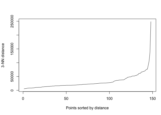

A little hard to see the knee, but I’m eyeballing 30000.

kNNdistplot(tor_dist, k = 3)
abline(h = 30000, lty = 3)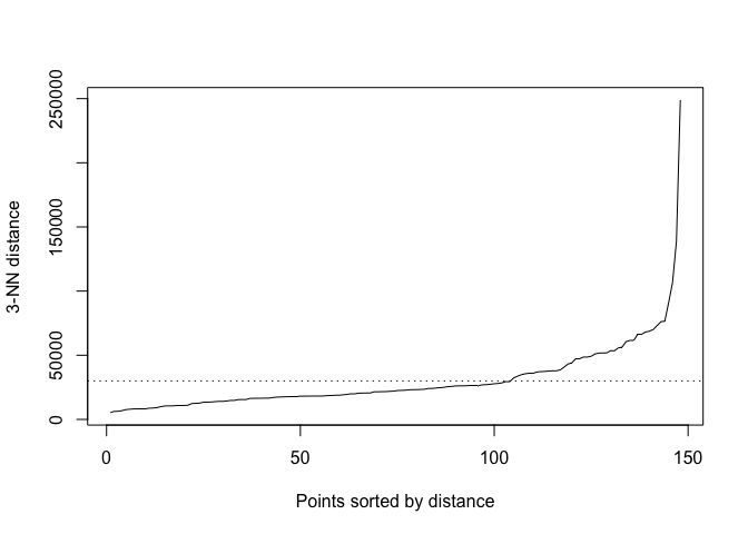

Now plug in minPts, Eps and your data frame of point coordinates into the function dbscan()

tor_dbscan <- dbscan(coords, eps = 30000, minPts = 4)

#also can use the distance matrix
#tor_dbscan <- dbscan(tor_dist, eps = 30000, minPts = 4)

The resulting object is a dbscan object.

class(tor_dbscan)

## [1] "dbscan_fast" "dbscan"

The cluster designations are saved in cluster.

table(tor_dbscan$cluster)

## 
##  0  1  2  3  4 
## 34 91  4 14  5

We find 4 tornado clusters. dbscan() designates noise points as 0. There are 34 noise points based on the parameters we chose. Note that the default in dbscan() assigns border points to the first cluster it is density reachable from. To consider all border points as noise, which is the DBSCAN* method proposed by Campello et al., (2015), set borderPoints = FALSE within dbscan().

Question 5: Create a dot map of the tornado points, using different colors or symbols to represent their DBSCAN cluster membership.

Question 6: Re-run DBSCAN for MinPts = 4 with Eps = 20000 and 40000. Re-run DBSCAN for MinPts = 7 and 10. Compare the number of clusters, the number of noise points and the location of clusters. Briefly explain the differences when you vary MinPts vs Eps.

Resources

The procedures in this lab heavily relies on the spatstat package, which is very well documented. Paula Moraga’s book has a few great chapters on spatial point patterns.

This work is licensed under a Creative Commons Attribution-NonCommercial 4.0 International License.

Website created and maintained by Noli Brazil

Point Pattern Analysis

GEO 200CN - Quantitative Geography

Professor Noli Brazil

May 4, 2026

Installing and loading packages

Why point pattern analysis?

Bringing in the data

Centrography

Density based measures

Overall density

Quadrat counts

Hypothesis testing

Kernel density

Distance based measures

Mean Nearest-Neighbor Distance

Hypothesis testing

Distance Functions

DBSCAN

Resources