Hypothesis Testing
GEO 200CN - Quantitative Geography
Professor Noli Brazil
April 13, 2026
In this lab guide, we’ll make statistical inferences about the significance of particular data values within a hypothesis testing framework. We will follow the material presented in this week’s lecture and handout.
The objectives of the guide are as follows
- Make inferences about the mean of one group (dependent samples)
- Make inferences about mean comparisons between two groups (independent samples)
We’ll use two data sets in this guide. The first contains current and forecasted climate values in Oregon. The second contains property values for buildings in Manhattan, New York City. The Oregon dataset will be used to accomplish objective 1, whereas the Manhattan dataset will be used to accomplish objective 2.
Loading packages
We’ll be using one package in this lab - tidyverse.
Load it in using library().
library(tidyverse)Dependent samples
Dependent sample hypothesis tests - also known as one-sample tests -
typically examine differences in the mean over time for the same sample.
Let’s bring in a data set that contains climate values (January and July
temperature and precipitation) simulated by a regional climate model for
present, and for potential future conditions when the concentration of
carbon dioxide in the atmosphere has doubled, for a set of model grid
points that cover Oregon. Read in the data set directly using
read_csv().
orsim <- read_csv("https://raw.githubusercontent.com/geo200cn/data/master/orsim.csv")The variables TJan1x, TJul1x, PJan1x and PJul1x are the simulated temperature (T) and precipitation (P) based on present carbon dioxide (C02) values, while the variables with 2x in their names are those for the doubled CO2 scenarios that are intended to describe the climate of the next century.
The research question is: How would a doubling of carbon dioxide in the atmosphere affect temperature over Oregon? From what we already know about the greenhouse effect, atmospheric change, and basic climatology, we can suspect that temperatures will increase with an increase in carbon dioxide. The question is, are the simulated temperatures for the enhanced greenhouse-situation significantly higher than those for present?
Before running any tests, let’s just look at the distribution of our two variables TJan2x and TJan1x. First, the mean difference.
mean(orsim$TJan2x) - mean(orsim$TJan1x)## [1] 4.089474Then histograms of each variable.
ggplot(orsim) +
  geom_histogram(mapping = aes(x=TJan1x))
ggplot(orsim) +
  geom_histogram(mapping = aes(x=TJan2x))
Remember what the Central Limit Theorem says?
Let’s do a side-by-side comparison using a boxplot. Do the groups visually differ?
orsim %>%
  select(TJan1x, TJan2x) %>%
  pivot_longer(cols = everything(),
               names_to = "variable",
               values_to = "value") %>%
  ggplot() +
  geom_boxplot(aes(x = variable, y = value)) +
ylab("Temperature") 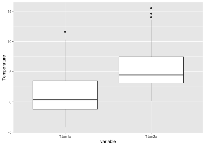
Descriptively, it looks like an increase in the mean temperature from present to future. But, let’s formally test it since we now have the tools to do so. Remember the steps in hypothesis testing outlined in the handout.
The null hypothesis is that there is no change or a decrease in temperature. The alternative hypothesis is that there is an increase in temperature.
We should not be fixated too much with threshold cutoffs, but the standard α is 0.05.
We’ll use the standard t statistic, which will allow us to conduct a t-test.
We’re computing a difference of means for paired observations, so this is a one-sample hypothesis test.
First, let’s calculate the difference between TJan2x and TJan1x and save it back in our data frame.
orsim <- orsim %>%
        mutate(diff = TJan2x - TJan1x)
Next, we calculate the standard error s. The function
length() gives you the total number of observations in the
dataset.
n <- length(orsim$diff)
s <-  sqrt(var(orsim$diff)) #formula from handout
Next, the t statistic
t1 = mean(orsim$diff)/(s/sqrt(n))  #formula from handout
t1
## [1] 192.6058pt().pt(t1, n-1, lower=FALSE)## [1] 2.141518e-144There is actually a canned function, t.test(), that you
can use to run the t-test. In the argument, we establish data
from the two time points. The argument paired = TRUE states
that the data are coming from the same sample. We establish the
alternative hypothesis by using the alternative argument.
alternative = "greater" is the alternative that the first
set of values has a larger mean than the second set of values. The
confidence level - or the significance threshold - is established using
the argument conf.level, which is 0.05, or 0.95.
t.test(orsim$TJan2x, orsim$TJan1x, paired = TRUE, alternative="greater", conf.level =.95)##
## Paired t-test
##
## data: orsim$TJan2x and orsim$TJan1x
## t = 192.61, df = 113, p-value < 2.2e-16
## alternative hypothesis: true mean difference is greater than 0
## 95 percent confidence interval:
## 4.054261 Inf
## sample estimates:
## mean difference
## 4.089474Similarly because this is basically a one-sample test, we can use the
diff
variable. alternative = "greater" is the alternative that
diff is
greater than 0.
t.test(orsim$diff, alternative="greater", conf.level =.95)##
## One Sample t-test
##
## data: orsim$diff
## t = 192.61, df = 113, p-value < 2.2e-16
## alternative hypothesis: true mean is greater than 0
## 95 percent confidence interval:
## 4.054261 Inf
## sample estimates:
## mean of x
## 4.089474Let’s have you complete this step.
Question 1: What is your conclusion regarding the difference between the present and simulated future January mean temperature over Oregon?
Question 2: How would you change the null and alternative hypotheses to make this a two-sided test? What is the p-value of this two-sided test?
Question 3: For January precipitation (PJan1x and PJan2x) test the hypothesis that PJan1x is less than PJan2x. Use a t-test with a 5% or 95% significance level. State the null and alternative hypotheses. Interpret your results.
Independent samples
To demonstrate independent samples or two-sample hypothesis testing,
let’s bring in the data set manhattan_buildings.csv, which
includes information about every building in Manhattan, over 40,000
buildings (wow!). Read in the data set directly using
read_csv()
MN<-read_csv("https://raw.githubusercontent.com/geo200cn/data/master/manhattan_buildings.csv")In a future lab you will start exploring spatial data in R. Although
MN is not spatialized, it does have spatial information,
longitude and latitude, which allows us to crudely plot it using our
friend ggplot().
##Map all of the buildings in Manhattan
ggplot(MN) +
    geom_point(mapping = aes(x = XCoord,
                             y = YCoord)) +
    xlab("Longitude") +
    ylab("Latitude")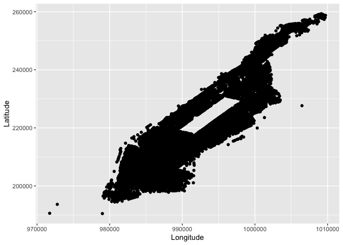
The research question is: Is there a difference in property values between buildings located in and out of historic districts? Historic neighborhoods are areas where the buildings have historical importance not because of their individual significance but because as a collection they represent the architectural sensibilities of a particular time period. They have tremendous historical and architectural value. But do they also carry greater financial value?
Before answering this question, we need to be able to identify buildings in historic districts. It looks like the variable HD gives us which district a building is located in
summary(MN$HD)## Min. 1st Qu. Median Mean 3rd Qu. Max.
## 0.0000 0.0000 0.0000 0.2531 1.0000 1.0000A variable that is coded 0,1 to refer to absence or presence,
respectively, is sometimes called a dummy variable or an indicator
variable. Although a dummy looks like a numeric, it is in fact a
qualitative or categorical variable (Yes/No). Since HD captures
whether a building is in or out of a historic district, we should tell R
that the numbers in the column are a code for historic districts, and we
do this by creating a factor, or categorical variable, using
as.factor(). A factor is a nominal (categorical) variable
with a set of known possible values called levels.
MN <- MN %>%
      mutate(HD = as.factor(HD))
Now we can draw a very crude map of buildings in historic districts.
ggplot(MN) +
    geom_point(mapping = aes(x = XCoord,
                             y = YCoord, col = HD)) +
    xlab("Longitude") +
    ylab("Latitude")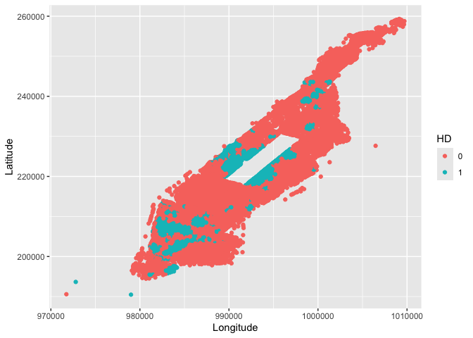
Finally, split the “MN” object into two tables, one for the historic buildings (inHD) and one for the buildings outside a historic district (outHD). We want to compare the mean property values for each these groups.
inHD <- MN %>%
  filter(HD == 1)

outHD <- MN %>%
  filter(HD == 0)
Our goal is to explore the effect of historic districts on property values in Manhattan. We want to find out if the designation of historic district has any effect on building property values. First, let’s create boxplots of property values, which are stored in the variable AssessTot, to see if there is a visual difference between the two groups.
ggplot(MN) +
  geom_boxplot(mapping = aes(x = HD, y=AssessTot)) +
  ylab("Assessment Value") +
xlab("In Historic District") 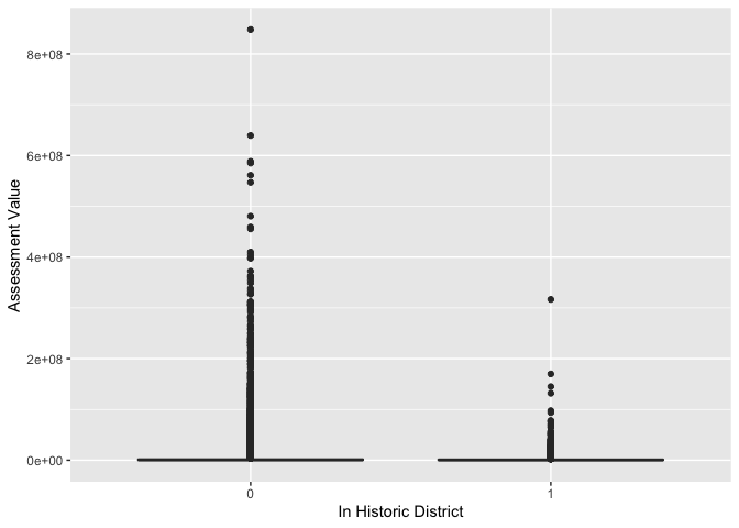
Next, we’ll use the function t.test() to run the
hypothesis test. In this case, x = is the data being
tested, y = is the comparison group (used for a two sample
test).
Question 4: Based on the research question, run the appropriate t-test using a 5% (or 95%) significance level to compare the mean property values of buildings in historic districts and those not in historic districts. State the null and alternative hypotheses. Briefly summarize your results.
In your training as a Geographer, you will find that one of the core tenets of the discipline is that location matter. Location is an important component of a property’s value. For example, we would expect property values for buildings in downtown Manhattan to be greater than buildings in a less wealthier area of the burrough. To test the impact of a historic district designation we should revise our test to examine only buildings that have similar locations. One way to do this is to identify buildings that are close to but outside of historic districts. Each building in the database has a block number. Let’s revise our dataset so that it only includes buildings which are on the same block as a historic district but outside of the district boundaries.
##Select buildings on the same block as a historic district
##Get a list of all blocks that contain historic buildings
blocks <- inHD$Block

#display the first 5 rows of blocks
head(blocks)
## [1] 7 72 73 29 7 29##Select all buildings (from MN) that are on the same block as historic buildings
##The line below selects all rows where the block column contains values in our list of blocks
##Save the result as a new object
HDB <- MN %>%
filter(Block %in% blocks)
HDB_out <- HDB %>%
filter(HD == 0)
HDB_in <- HDB %>%
filter(HD == 1)Now we have two files that contain buildings on blocks with historic districts, one file describes buildings in the district and the other describes those outside the district boundaries. But, we need one more correction: size. The size of the building is an important determinant of its value. The variable AssessSqFt is the assessed value per square foot. We want to run a t-test to compare the mean property values per square footage of buildings in historic districts and those not in historic districts (for those in the same blocks).
Question 5: Based on the research question, run the appropriate t-test (using a 5% or 95% significance level) to compare the mean property values per square footage of buildings in historic districts and those not in historic districts. State the null and alternative hypotheses. Summarize your results.

This
work is licensed under a
Creative
Commons Attribution-NonCommercial 4.0 International License.
Website created and maintained by Noli Brazil